Volatility Interface to BAP

Note: libbap will fail to load in environments that can not import volatility.obj. For this reason, you might find it useful to experiment with libbap from the Volatility shell (i.e. volshell) rather than from a Python command line prompt.

Basics

Code that you wish to analyse (either manually or programmatically) is encapsulated by a Program object instance as follows:

Volshell> from bap import *                 # Load libbap and along with its commands and helper functions

Volshell> arch = "x86"                      # String holding the CPU architecture (x86 and amd are possible)
Volshell> code1 = "AAAA"                    # Python string holding the binary x86 code
Volshell> addr = 0xdeadbeef                 # Address at which the x86 code is located in process memory
Volshell> prog1 = Program(arch, code1, addr)

Object creation parses the supplied binary code to produce a (hidden) immutable BAP IL term. By default, the object instance has the following methods:

• __str__ this method returns a Python string representing the encapsulated BAP IL term
• __call__ this method takes a list of BAP commands and processes them in turn (as the BAP IL term is immutable, it is not permanently altered by this processing).

BAP IL terms may be in one of three possible forms:

• Abstract syntax tree (AST) this is the initial or default form of a BAP IL term - use to_ast() to convert to this form
• Control-flow graph (CFG) see the relevant subsection below - use to_cfg() to convert to this form
• Static-single analysis graph (SSA) see the relevant subsection below - use to_ssa() to convert to this form.

A selection of Python commands to transform, analyse and convert the encapsulated BAP IL term have been defined (commands can only be applied to BAP IL terms in the appropriate form). For example, to print out the BAP IL AST:

Volshell> prog1(pp_ast())         # AST printed to stdout (same as 'print str(prog1)')
Volshell> prog1(pp_ast("bap.il")) # textual version of AST saved in file bap.il

addr 0xd4@asm "inc    %ecx"
label pc_0xd4
T_t:u32 = R_ECX:u32
R_ECX:u32 = R_ECX:u32 + 1:u32
R_OF:bool = high:bool((T_t:u32 ^ -2:u32) & (T_t:u32 ^ R_ECX:u32))
R_AF:bool = 0x10:u32 == (0x10:u32 & (R_ECX:u32 ^ T_t:u32 ^ 1:u32))
R_PF:bool =
  ~low:bool(R_ECX:u32 >> 7:u32 ^ R_ECX:u32 >> 6:u32 ^ R_ECX:u32 >> 5:u32 ^
            R_ECX:u32 >> 4:u32 ^ R_ECX:u32 >> 3:u32 ^ R_ECX:u32 >> 2:u32 ^
            R_ECX:u32 >> 1:u32 ^ R_ECX:u32)
R_SF:bool = high:bool(R_ECX:u32)
R_ZF:bool = 0:u32 == R_ECX:u32
addr 0xd5@asm "inc    %ecx"
label pc_0xd5
T_t_82:u32 = R_ECX:u32
R_ECX:u32 = R_ECX:u32 + 1:u32
R_OF:bool = high:bool((T_t_82:u32 ^ -2:u32) & (T_t_82:u32 ^ R_ECX:u32))
R_AF:bool = 0x10:u32 == (0x10:u32 & (R_ECX:u32 ^ T_t_82:u32 ^ 1:u32))
R_PF:bool =
  ~low:bool(R_ECX:u32 >> 7:u32 ^ R_ECX:u32 >> 6:u32 ^ R_ECX:u32 >> 5:u32 ^
            R_ECX:u32 >> 4:u32 ^ R_ECX:u32 >> 3:u32 ^ R_ECX:u32 >> 2:u32 ^
            R_ECX:u32 >> 1:u32 ^ R_ECX:u32)
R_SF:bool = high:bool(R_ECX:u32)
R_ZF:bool = 0:u32 == R_ECX:u32
addr 0xd6@asm "inc    %ecx"
label pc_0xd6
T_t_83:u32 = R_ECX:u32
R_ECX:u32 = R_ECX:u32 + 1:u32
R_OF:bool = high:bool((T_t_83:u32 ^ -2:u32) & (T_t_83:u32 ^ R_ECX:u32))
R_AF:bool = 0x10:u32 == (0x10:u32 & (R_ECX:u32 ^ T_t_83:u32 ^ 1:u32))
R_PF:bool =
  ~low:bool(R_ECX:u32 >> 7:u32 ^ R_ECX:u32 >> 6:u32 ^ R_ECX:u32 >> 5:u32 ^
            R_ECX:u32 >> 4:u32 ^ R_ECX:u32 >> 3:u32 ^ R_ECX:u32 >> 2:u32 ^
            R_ECX:u32 >> 1:u32 ^ R_ECX:u32)
R_SF:bool = high:bool(R_ECX:u32)
R_ZF:bool = 0:u32 == R_ECX:u32
addr 0xd7@asm "inc    %ecx"
label pc_0xd7
T_t_84:u32 = R_ECX:u32
R_ECX:u32 = R_ECX:u32 + 1:u32
R_OF:bool = high:bool((T_t_84:u32 ^ -2:u32) & (T_t_84:u32 ^ R_ECX:u32))
R_AF:bool = 0x10:u32 == (0x10:u32 & (R_ECX:u32 ^ T_t_84:u32 ^ 1:u32))
R_PF:bool =
  ~low:bool(R_ECX:u32 >> 7:u32 ^ R_ECX:u32 >> 6:u32 ^ R_ECX:u32 >> 5:u32 ^
            R_ECX:u32 >> 4:u32 ^ R_ECX:u32 >> 3:u32 ^ R_ECX:u32 >> 2:u32 ^
            R_ECX:u32 >> 1:u32 ^ R_ECX:u32)
R_SF:bool = high:bool(R_ECX:u32)
R_ZF:bool = 0:u32 == R_ECX:u32

Each Python command is implemented as a function that returns a list (of internal actions). This allows multiple commands to be easily chained together using Python's append (i.e. +) operator. For example, to print out the CFG for the BAP IL term:

Volshell> prog1(to_cfg()+pp_cfg())          # convert BAP IL (AST) to CFG and view via xdot
Volshell> prog1(to_cfg()+pp_cfg("cfg.dot")) # dot version of CFG saved in file cfg.dot

By default, BAP CFGs contain an indirect graph node to over approximate indirect jumps during analysis. These may be removed using the rm_indirect_cfg() or prune_cfg() commands as follows:

Volshell> prog1(to_cfg()+rm_indirect_cfg()+pp_cfg()) # CFG, but with no indirect graph node
Volshell> prog1(to_cfg()+prune_cfg()+pp_cfg()) # CFG, but with no indirect or error graph nodes

This trick is sometimes useful when you wish to annotate a CFG with constraints and then require an AST form for solving the constraints (see the Constraint Solving subsection).

Command Help

Help information regarding BAP commands can be generally viewed using any of the following:

Volshell> help(commands) # Generic BAP commands
Volshell> help(analysis) # Miscellaneous abstract interpretation commands
Volshell> help(stp)      # Theorem prover/solver commands
Volshell> help(vc)       # Verification condition (i.e. WP) commands

Volshell> help(pp_ast)
Volshell> help(to_cfg)

Programmatic Interaction with BAP

Sometimes, we would like to take the results of running various BAP commands (e.g. the result of a program slice or an invalidating model assignment), and then use Python code to generate new BAP analysis commands.

In order to do this, it is necessary for the BAP commands to return Python data structures (rather than generate DOT or textual output).

Using the command return_term(), BAP commands can be made to return a Python dictionary data structure. This dictionary has the following keys:

• term this key returns a Python data structure that encodes the resulting AST IL term or CFG/SSA graphs
• model when present, this key returns a Python dictionary encoding the resulting interpretation (BAP variables are mapped to integer values)
• wp when present, this key returns a Python dictionary holding the WP pre-condition (use key pre) and a list of universally quantified variables (use key foralls)

Note: return_term() causes the entire BAP command list to be evaluated, and it is the result of this that is returned.

Viewing Graphs

Control-flow Graphs

Control-flow graphs (CFGs) are directed graphs showing how the binary code might be traversed during execution. BAP CFGs have nodes that are lists of instructions (c.f. blocks) and edges indicate where control leads to next on leaving a node. Edges may be labelled with booleans indicating a conditional transfer of control (in BAP CFGs: blue edges are unlabelled; green edges are labelled true; and red edges are labelled false).

Some of BAPs commands will only process CFGs. Should this be the case, and an incorrectly typed BAP object is passed to the command, then an error message telling you to convert to the (AST) CFG format is generated. For example:

Volshell> prog1(analysis.struct()) # results in 'RuntimeError: Failure("need explicit translation to AST CFG")'

Structure analysis (see Advanced compiler design and implementation by Steven S Muchnick) allows a CFG to be analysed so as to identify its control-flow structure (i.e. identify nested blocks, if-thens, if-then-elses, while-loops, etc. using a graph term reduction strategy). The following shows how we may do this in BAP:

Volshell> code2 = "\x81\xce\xff\x00\x00\x00\x46\x66\x81\xfe\x00\x04\x77\xf2"
Volshell> prog2 = Program(arch, code2, addr)
Volshell> prog2(to_cfg()+analysis.struct()+pp_cfg())

Note: the underlying structural analysis code appears to have issues identifying some conditional statements, and so loop structures.

Static-single Analysis Graphs

Static-single analysis graphs (SSAs) are CFGs, but all variables are assigned to at most once. This type of graph is generated by splitting multiply assigned variables of the CFG into different versions (hence why variables end up with integer prefixes).

When alternative paths (e.g. of a conditional) assign to the same variable, phi-nodes are introduced to merge these information flows.

SSAs make use-def chains explicit and simplify the presentation of some abstract interpretations.

Graph Manipulations

CFGs and SSAs identify their nodes by their basic block ID (BBID). BBIDs are used to label each node and are of one of the following forms:

• BB_Entry identifies the basic block or node that we start executing with
• BB_Exit indicates the basic block or node that we normally exit from
• BB_Error indicates the basic block or node that we enter should an error (e.g. invalid jump address), exception, etc. occur during execution
• BB_indirect indicates the basic block or node that calculated jumps or returns should go to (these nodes over approximate the real semantics)
• BB_XXXX indicates a general basic block or node holding code that is to be executed.

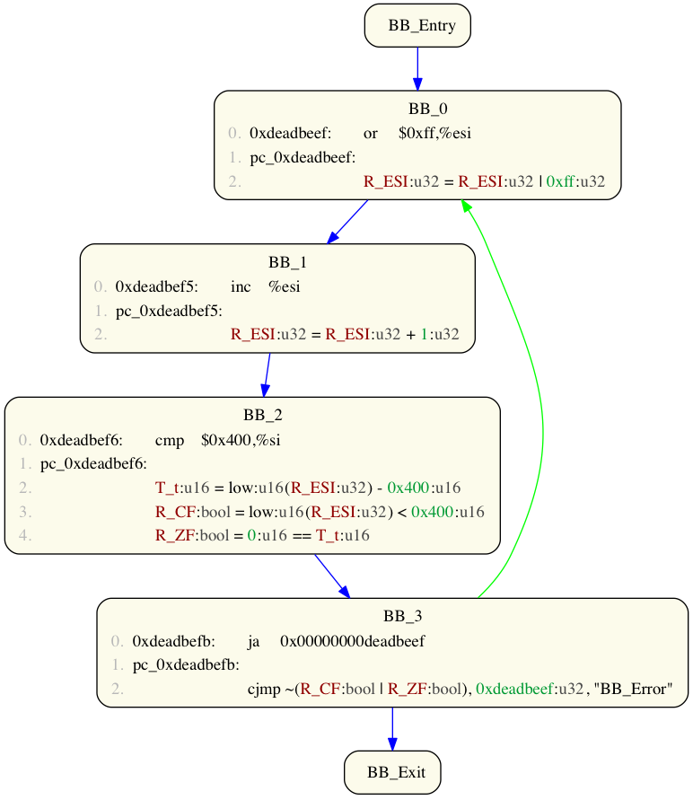
Basic blocks hold a list of BAP IL terms. Terms within a given basic block are identified using the line number (starting at zero) at which the term occurs (look for the light grey numbers on the left of the graph nodes). For example, in the following CFG, the highlighted BAP IL term is referenced as line number 4 of BBID BB_1:

Working with Loops and Cycles

A number of BAPs analyses (e.g. weakest pre-conditions and value-set analysis) are implemented to only handle straight line or sequential code. Thus it is often necessary to iteratively approximate loop behaviour by unrolling loops and then eliminating any remaining cycles. The following BAP commands support such manipulations:

• unroll(n) unrolls loops in a CFG n times
• rm_cycles() removes cycles from the CFG.

For example, consider the following CFG:

We can approximate this CFGs looping behaviour by unrolling the loop 4 times:

Volshell> prog2(to_cfg()+prune_cfg()+unroll(4)+pp_cfg())

Note: it is important to prune out unreachable graph nodes (e.g. indirect and error nodes), otherwise unrolling will fail.

This yields the following expanded CFG:

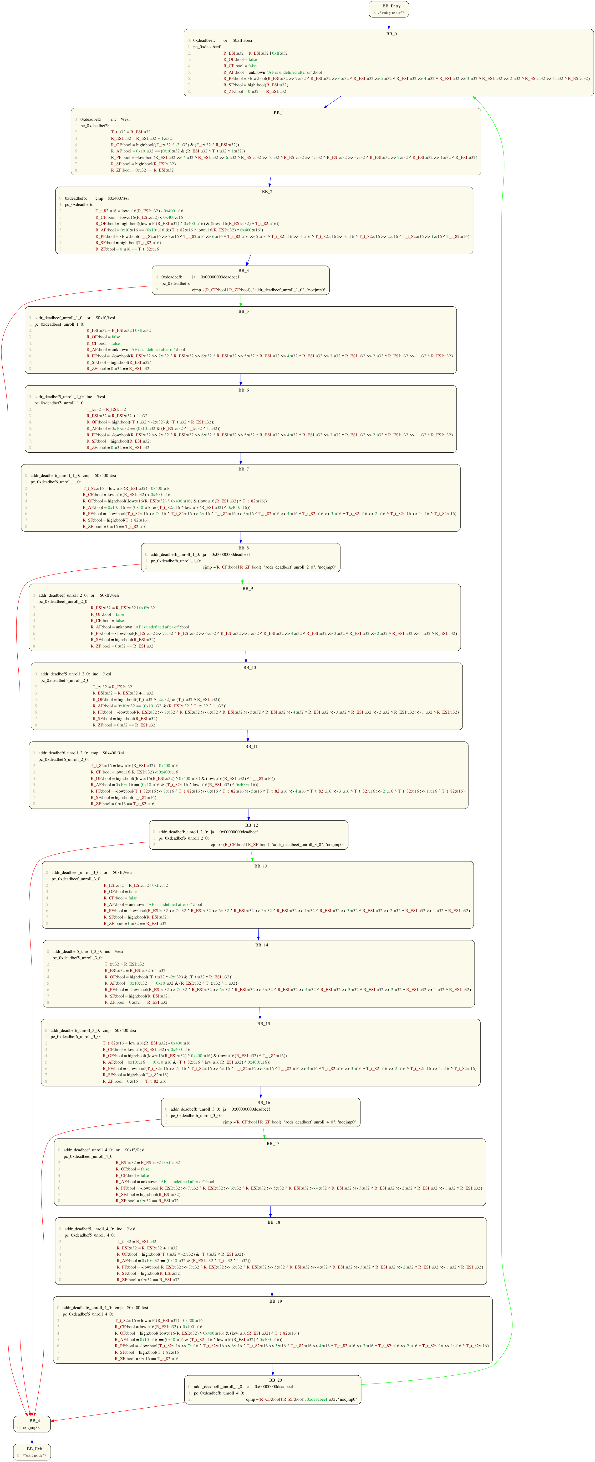
We can now further investigate this unrolled CFG by examining the exit conditions for each of the 5 ja 0xdeadbeef nodes. Either removing cycles (to get an acyclic CFG) or program slicing can help in doing this.

Program Slicing

Often, when analysing code, we have a statement of interest and we would like to know what other statements it depends upon. For example, consider the following CFG:

Imagine we wish to understand something regarding the conditions under which the loop terminates. We perform a program slice from line 0 of BBID BB_0 (the loop's entry point) to line 2 of BBID BB_3 (the loop's exit point):

Volshell> prog2(to_cfg()+slice_cfg(0, 0, 3, 2)+pp_cfg())

Notice how we have simplified the graph to just those elements of the loop body required to calculate our termination/looping condition.

Note: if you choose a slice end point that is not a move or jump IL term, then you will get a graph devoid of any IL terms!

Assertions and Assumptions

Sometimes, when working with code we know something about the contextual conditions in which the code will execute. BAP allows us to model this by adding in assert and assume terms.

Asserts express predicates that are to be model checked at a given execution point (these get added as conclusions to generated VCs). Whilst assumes express predicates that the model checker assumes as holding at that execution point (these get added as assumptions to generated VCs).

Consider the following CFG:

and assume we know that, upon entry to the graph, R_ECX is a multiple of 4. The following BAP term expresses this fact:

R_ECX:u32 % 4:u32 == 0:u32

We can add this expression as an assume statement into our CFG as follows:

Volshell> prog1(to_cfg()
                +add_assume("R_ECX:u32 % 4:u32 == 0:u32", "BB_Entry", 0)
                +pp_cfg())

We expect that, upon exit, the same predicate will hold. We can also add this in to our CFG via an assert statement as follows:

Volshell> prog1(to_cfg()
                +add_assume("R_ECX:u32 % 4:u32 == 0:u32", "BB_Entry", 0)
                +add_assert("R_ECX:u32 % 4:u32 == 0:u32", "BB_Exit", 0)
                +pp_cfg())

Latter (see the Constraint Solving subsection), we will look at how this code invariant can be automatically proved true using SMT theorem prover support (i.e. STP, CVC3, YICES or Z3).

Calculating Weakest Pre-conditions

Sometimes, we know that some predicate holds at BB_Exit. This predicate is our post condition and can be asserted using the BAP command stp.post(post_pred).

Given a post condition, a natural question to ask is what are the minimal logical conditions that must hold at BB_Entry in order for this post condition to hold. This minimal logical condition is known as a weakest pre-condition (WP) and the Python vc package provides a number of BAP commands for calculating these.

Using stp.solve(validity=False) (or, more simply, stp.solve()) we can check satisfiability of wp => post_pred (where wp is the calculated WP). In doing this, the model interpretations returned here provides initial conditions under which the code can run in order to satisfy the post-condition.

Note: the following Python helper functions are provided to aid in working with WPs:

• vclist() returns a list of supported Verification Condition (VC) commands.
• pred_vclist() returns a list of supported Verification Condition (VC) commands that only require predicate logic (i.e. no quantifiers).

Constraint Solving

Using SMT theorem prover support (i.e. STP, CVC3, YICES or Z3), it is possible to take BAP ASTs and generate interpretations (i.e. maps/dictionaries assigning integer values to variables) or to validate the AST term.

We have already seen (see the Assertions and Assumptions subsection) how CFGs may be annotated with assert and assume predicates (c.f. program constraints). If we convert the annotated AST term into a CFG, we may then use BAP's solver interface to show the term is valid or to generate counter examples (in the form of a counterexample interpretation).

Note: the following helper functions are supplied to aid in working with BAP IL variable expressions:

• x86_regs() returns the BAP IL variables used to model the x86 registers
• x86_mem() returns the BAP IL variables used to model x86 memory
• amd_regs() returns the BAP IL variables used to model the AMD registers
• all_regs() returns the result of all of the above functions
• get_x86_var(reg) returns the BAP IL variable corresponding to a given x86 register
• get_amd_var(reg) returns the BAP IL variable corresponding to a given AMD register
• var_to_str(var) returns a string representation of the given BAP IL variable (this string is typically the variable name appended by its unique hash value).

Example 1

The following BAP commands generate a CFG with the BB_Entry and BB_Exit blocks annotated with a predicate constraining R_ECX to be a multiple of 4:

Volshell> prog1(to_cfg()
                +add_assume("R_ECX:u32 % 4:u32 == 0:u32", "BB_Entry", 0)
                +add_assert("R_ECX:u32 % 4:u32 == 0:u32", "BB_Exit", 0)
                +pp_cfg())

We would like to be able to show that this constraint annotated CFG is (provably) valid. To do this, we first remove the indirect node and then apply BAP's solver as follows:

Volshell> prog1(to_cfg()
                +add_assume("R_ECX:u32 % 4:u32 == 0:u32", "BB_Entry", 0)
                +add_assert("R_ECX:u32 % 4:u32 == 0:u32", "BB_Exit", 0)
                +rm_indirect_cfg()+to_ast()+stp.solve(validity=True))

Applying optimizations...
Ssa_Simp: Starting iteration 0
Deadcode: Dead var R_AF_12:bool is undefined
Deadcode: Dead var R_CF_10:bool is undefined
Deadcode: Dead var T_t_761:u16 is undefined
Deadcode: Dead var R_ESI_2:u32 is undefined
Deadcode: Dead var R_SF_14:bool is undefined
Deadcode: Dead var R_ZF_13:bool is undefined
Deadcode: Dead var R_PF_11:bool is undefined
Deadcode: Dead var R_OF_15:bool is undefined
Deadcode: Dead var T_t_760:u32 is undefined
Deadcode: Deleting 96 dead stmts
Ssa_Simp: Starting iteration 1
Deadcode: Deleting 0 dead stmts
Computing predicate...
Printing predicate as BAP expression
let temp_3239:bool := R_ECX_7:u32 % 4:u32 == 0:u32 in
~temp_3239:bool | temp_3239:bool & true
Printing predicate as SMT formula
Stp: Computing freevars...
Solving
Solve result: Valid

Here we see that the configured SMT prover has validated our constrained CFG - i.e. prog1 preserves the data invariant R_ECX:u32 % 4:u32 == 0:u32.

As contrast, consider the following alternative session where we annotate the BB_Exit node with an invalid constraint:

Volshell> prog1(to_cfg()+rm_indirect_cfg()
                +add_assume("R_ECX:u32 % 4:u32 == 0:u32", "BB_Entry", 0)
                +add_assert("R_ECX:u32 % 4:u32 == 1:u32", "BB_Exit", 0)
                +to_ast()+stp.solve(validity=True))

Applying optimizations...
Ssa_Simp: Starting iteration 0
Deadcode: Dead var R_AF_12:bool is undefined
Deadcode: Dead var R_CF_10:bool is undefined
Deadcode: Dead var T_t_761:u16 is undefined
Deadcode: Dead var R_ESI_2:u32 is undefined
Deadcode: Dead var R_SF_14:bool is undefined
Deadcode: Dead var R_ZF_13:bool is undefined
Deadcode: Dead var R_PF_11:bool is undefined
Deadcode: Dead var R_OF_15:bool is undefined
Deadcode: Dead var T_t_760:u32 is undefined
Deadcode: Deleting 95 dead stmts
Ssa_Simp: Starting iteration 1
Deadcode: Deleting 0 dead stmts
Computing predicate...
Printing predicate as BAP expression
let temp_3140:u32 := R_ECX_7:u32 % 4:u32 in
~(temp_3140:u32 == 0:u32) | temp_3140:u32 == 1:u32 & true
Printing predicate as SMT formula
Stp: Computing freevars...
Solving
Model:
R_ECX_7 -> 0
Solve result: Invalid

Here we see that by starting prog1 in a state where R_ECX contains 0 (using x86_regs() we determine that R_ECX_7 is the entry value for the R_ECX register), we will end in a state that invalidates the BB_Exit constraint (i.e. R_ECX:u32 % 4:u32 == 1:u32 is falsified).

Note: in the textual output, the model displays integers in hex.

This interpretation may be extracted programmatically in Python as follows:

Volshell> prog1(to_cfg()+rm_indirect_cfg()
                +add_assume("R_ECX:u32 % 4:u32 == 0:u32", "BB_Entry", 0)
                +add_assert("R_ECX:u32 % 4:u32 == 1:u32", "BB_Exit", 0)
                +to_ast()+stp.solve(validity=True)+return_term())['model']

{'R_ECX_7': '0'}

Example 2

In the subsection Working with Loops and Cycles, we looked at unfolding prog2 in the following manner:

Volshell> prog2(to_cfg()+prune_cfg()+unroll(4)+rm_cycles()_pp_cfg())

We can now show that, whenever R_ESI at BB_Entry has its low word in the range [0x0, 0x400), then byte 1 of R_ESI will be in the range (0, 4]. This is shown by inserting an assumption and an assertion into our CFG and then validating with the configured solver as follows:

Volshell> prog2(to_cfg()+prune_cfg()+unroll(4)+rm_cycles()
                +add_assume("low:u16(R_ESI:u32) < 0x400:u16", "BB_Entry")
                +add_assert("0x0:u8 < high:u8(low:u16(R_ESI:u32)) & high:u8(low:u16(R_ESI:u32)) <= 0x4:u8 ")
                +to_ast()+stp.solve(validity=True))

However, establishing that whenever:

0x400:u16 <= low:u16(R_ESI:u32)

high:u8(low:u16(R_ESI:u32)) == 0:u8

Using Abstract Interpretation

BAP provides the OCaml signature file ocaml/graphDataflow.mli with which abstract interpretations may be implemented.

usedef and defuse Chains

The BAP commands analysis.usedef() and analysis.defuse() may be used to extract use-def and def-use chains. The results of these chains can be extracted as a Python data structure using the return_term() command.

Value-set Analysis

Value-set analysis (VSA) can be performed using the analysis.vsa() command. This command annotates an SSA graph with the results of the analysis. The results of this analysis can be extracted as a Python data structure using the return_term() command - here one extracts the VSA analysis from the Python encoding of the SSA graph.

Unfortunately, VSA (as implemented) can not handle program loops. Moreover, the current VSA implementation does not take into account assert and assume statements. As a result, the value of this analysis is currently limited.

Generating and Instrumenting LLVM Bitcode

Using the BAP codegen command, it is possible to take BAP IL terms and generate LLVM bitcode. For memory accesses, this may be done in such a way that:

• reads and writes occur directly to memory
• reads and writes are replaced by calls to the Python functions get_memory(addr) (which should return the memory contexts at addr) and set_memory(addr, val) (which should return a Python boolean indicating if the write succeeded or not).

For example, to generate LLVM bitcode from x86 code (without instrumenting memory) use the following:

Volshell> code1(codegen("code1.bc"))

The output file code1.bc may then be ran using llvm-mc.

Note: system calls (i.e. specials) are not currently handled by the BAP Llvm_codegen module.

TODO: ensure following actually works!

In order to generate instrumented LLVM bitcode from x86, use the following:

Volshell> code1(codegen("instrumented-code1.bc", get_memory=instrumented_read, set_memory=instrumented_write))

where our Python instrumentation functions are here defined by:

def instrumented_read(vol_obj, addr):
  val = vol_obj.get_memory(addr)
  print "RD: 0x{08x:0} -> {1}".format(addr, val)
  return val                            # "hook" reads and print out some debugging information

def instrumented_write(vol_obj, addr, val):
  print "WR: {1} -> 0x{08x:0}".format(addr, val)
  return vol_obj.set_memory(addr, val)  # "hook" writes and print out some debugging information