Wiki
Clone wikiwapor-et-look / WaPOR_data_components_and_methodology / AETI
Evapotranspiration (AETI), Land Cover Classification (LCC), Net Primary Productivity (NPP), Precipitation (PCP), Phenology (PHE), Quality layers (QUAL), Reference Evapotranspiration (RET), Soil moisture (RSM), Total Biomass Production (TBP) and Water Productivity (WP)
Evapotranspiration data components: E, T and I
Evapotranspiration is the sum of the soil evaporation (E), canopy transpiration (T) and interception (I). The interception describes the rainfall intercepted by the leaves of the plants that will be directly evaporated from their surface. The Evaporation, Transpiration and Interception are limited by climate (wind speed, radiation and air temperature) and soil conditions (soil moisture content). The sum of all three parameters i.e. the Actual Evapotranspiration and Interception (ETIa) can be used to quantify the agricultural water consumption. In combination with biomass production or yield it is possible to derive the agricultural water productivity.
WaPOR data components
The evapotranspiration data components (E, T, I) are produced using the same processing chain at all resolution levels. The data are delivered at a dekadal basis at all levels where pixel values represent the average daily E, T, I and ETIa values for that specific dekad in mm/day. The WaPOR database also provides monthly and annual sums.
Table x: Overview of E, T, I and ETIa data components
| Data component | Unit | Range | Use | Temporal resolution |
|---|---|---|---|---|
| Evaporation | mm/day mm/year |
0-2 - |
Measures soil evaporation in a dekad Accumulated soil evaporation over a year |
dekadal annual |
| Transpiration | mm/day mm/year |
0-10 - |
Measures canopy transpiration in a dekad Accumulated canopy transpiration over a year |
dekadal annual |
| Interception | mm/day mm/year |
0-2 - |
Measures canopy interception in a dekad Accumulated canopy interception over a year |
dekadal annual |
| Actual evapotranspiration and interception (ETIa) | mm/day mm/year |
0-12 - |
Can be used to quantify the agricultural water consumption. In combination with biomass production or yield, it is possible to derive the agricultural water productivity. Accumulated ETIa over a year |
dekadal annual |
Average daily E, T, I and ETIa values can be converted into volume for a specific area, e.g. 1 mm = 1 l/m2 or 1 mm = 10 m3/ha. The range of values for evaporation is for land, on open water, one would find values up to 15 mm/day.
Methodology
The method to calculate E and T is based on the ETLook model described in Bastiaanssen et al. (2012). It uses the Penman-Monteith (P-M) equation, adapted to remote sensing input data.
The Penman-Monteith equation (Monteith, 1965) predicts the rate of total evaporation and transpiration using commonly measured meteorological data (solar radiation, air temperature, vapour pressure and wind speed). It has become the FAO standard for calculating the actual and reference evapotranspiration. FAO irrigation and drainage paper 56 (Allen et al., 1998) describes the method in detail . The reader is advised to consult this document for detailed information on the use of the P-M equation and guidelines regarding the calculation of evapotranspiration.
The Penman-Monteith equation is also known as the combination-equation because it combines two fundamental approaches to estimate evaporation (Allen et al., 2005). These are the surface energy balance equation and the aerodynamic equation. The Penman-Monteith equation is expressed as:

where:
λ = latent heat of evaporation [J kg-1]
E = evaporation [kg m-2 s-1]
T = transpiration [kg m-2 s-1]
Rn = net radiation [W m-2]
G = soil heat flux [W m-2]
ρa = air density [kg m-3]
cp = specific heat of dry air [J kg-1 K-1]
ea = actual vapour pressure of the air [Pa]
es = saturated vapour pressure [Pa] which is a function of the air temperature
Δ = slope of the saturation vapour pressure vs. temperature curve [Pa K-1]
γ = psychrometric constant [Pa K-1]
ra = aerodynamic resistance [s m-1]
rs = bulk surface resistance [s m-1]
The ETLook model solves two versions of the P-M equation: one for the soil evaporation (E) and one for the canopy transpiration (T):

and

The two equations differ with respect to the net available radiation (Rn,soil and Rn,canopy) as well as the aerodynamic and surface resistance (ra,soil, rs,soil and ra,canopy,rs, canopy). Furthermore, the soil heat flux (G) is not taken into account for transpiration.
The Net Radiation and the Aerodynamic and Surface Resistance are discussed in more detail below. The other parameters of the equation are not taken into further consideration, as these are constants or variables that can be derived directly from mathematical relationships.
The main concepts of the ETLook model are illustrated in the schematic representation below.

Figure x: Schematic diagram illustrating the main concepts of the ETLook model, where two parallel Penman-Monteith equations are solved. For transpiration the coupling with the soil is made via the subsoil or root zone soil moisture content whereas for evaporation the coupling is made via the soil moisture content of the topsoil. Interception is the process where rainfall is intercepted by the leaves and evaporates directly from the leaves using energy that is not available for transpiration.
Net radiation
The net radiation Rn represents the available energy at the earth’s surface, which can be described by the radiation balance:

where α0 is the surface albedo [-], Rs is incoming solar radiation [W m-2], L* is net long wave radiation [W m-2], I represents energy dissipation due to interception losses [W m-2].
The net radiation is derived differently for the soil and canopy. Leaf area index Ilai, a measure of canopy density, is used to separate the net radiation into soil net radiation and canopy net radiation. An increase in leaf area index results in an exponential decrease in the fraction of the radiation available for the soil as more is captured by the canopy. The division is calculated using Beer’s law (which describes the attenuation of light through a material), leading to the following descriptions of soil and canopy net radiation:


where a is the light extinction factor for net radiation [-].
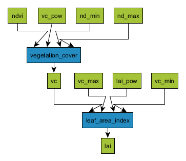
The leaf area index (LAI) Ilai [m2m-2] describes the amount of green leaf area per unit of soil area. A leaf area index equal to zero indicates that there is no vegetation present, a leaf area index larger than zero indicates the presence of green leaves. The NDVI Indvi [-] is used to derive\ Ilai. This is done in two steps. First, NDVI is used to calculate vegetation cover cveg, which is subsequently converted into leaf area index. The two equations below describe this conversion for a specific range of the NDVI value.

The constant nd_{max} is set at 0.91 for L1 300m data, and at 0.85 for L2 100m and L3 20m data.
The second step is the conversion from vegetation cover to leaf area index Ilai according to the following relationships:

This relationship has been derived using a large number of LAI functions compiled from literature (e.g. Carlson and Ripley, 1997; Duchemin, et al., 2006). The above relationship represents the average from these compiled relationships.
Interception is the process where rainfall is intercepted by the leaves. This evaporates directly from the leaves and requires energy that is not available for transpiration. Interception I [mm day-1] is a function of the vegetation cover, LAI and precipitation (P), expressed as (Hoyningen-Hüne, 1983, Braden, 1985):

Interception is relatively high with a small amount of precipitation, with the fraction intercepted decreasing quickly as precipitation increases. The maximum interception is determined by the LAI. The energy I needed to evaporate I_{mm} is calculated as follows:

where:
λ latent heat of evaporation [J kg-1]
The net long wave radiation L*, i.e. the difference between the incoming and outgoing long wave radiation, is computed using the formulation described in FAO report no 56 (Allen et al., 1998). This is a function of the air temperature (Ta), actual vapour pressure (ea) and transmissivity (τ).
As indicated above, the total evapotranspiration is obtained by summing the soil evaporation and canopy transpiration calculated from the Penman-Monteith equation and the interception by the leaves.
Soil heat flux (G)
The soil heat flux G is required to calculate evaporation from the soil surface. It is calculated according to FAO report no 56 (Allen et al., 1998). For northern latitudes, the maximum value for G is recorded in May. For southern latitudes this occurs in November. For northern latitudes it is calculated with the equation below. -π/4 is replaced by 3π/4 for southern latitudes.

where:
At,year = yearly air temperature amplitude [K]
k = soil thermal conductivity [W m-1 K-1]
J = day of year [-]
p = number of days in year [-]
zd = damping depth [m]
Ilai = leaf area index [-]
α = light extinction factor for net radiation [-]
The damping depth (zd) and the soil thermal conductivity (k) depend on soil characteristics. Usually these are taken as constants. The yearly air temperature amplitude is derived from climatic data.
Surface resistances (rs)
The surface resistances in the Penman-Monteith equations describe the influence (resistance) of the soil and the canopy on the flow of vapour in relation to evaporation and transpiration.
The soil resistance rs,soil is modelled using the minimal soil resistance rsoil,min and relative soil moisture content Se by means of a constant power function (Camillo and Gurney, 1986; Clapp and Hornberger, 1978; Dolman, 1993; Wallace et al., 1986):

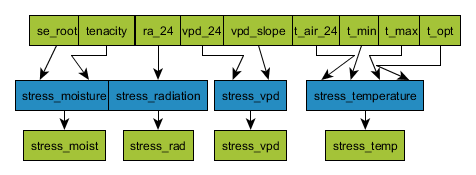
The canopy resistance is a function of the leaf area index, minimum stomatal resistance rcanopy,min and a number of reduction factors (Jarvis, 1976; Stewart, 1988). The Jarvis-Stewart parameterization describes the joint response of soil moisture and LAI on transpiration considering meteorological conditions (solar radiation, temperature and relative humidity φ):

where:
rcanopy,min = minimum stomatal resistance [s m-1]
Ilai,eff = effective leaf area index [-]
St = temperature stress [-], a function of minimum, maximum and optimum temperatures as defined by Jarvis (1976)
Sv = vapour pressure stress induced due to persistent vapour pressure deficit [-]
Sr = radiation stress induced by the lack of incoming shortwave radiation [-]
Sm = soil moisture stress originating from a lack of soil moisture in the root zone [-]
The minimum stomatal resistance rcanopy,min can have different values for different types of vegetation. This is derived from land cover information. The canopy resistance equation is based on a single leaf layer, therefore effective leaf area index has to be calculated as follows (Mehrez et al., 1992; Allen et al., 2006a):

Aerodynamic resistance (ra)
The aerodynamic resistance determines the transfer of heat and water vapour from the evaporating surface into the air above the canopy. The aerodynamic resistance has to be calculated for both neutral and non-neutral conditions. Neutral conditions exist when turbulence is created by shear stress (wind) only. Buoyancy (thermal rise of air) causes unstable non-neutral conditions. Under neutral conditions the aerodynamic resistance for soil (ra,soil) and canopy (ra,canopy) can be computed (Allen et al., 1998; Choudhury et al., 1986; Holtslag, 1984) with:


Where:
k = von Karman constant [-]
uobs = wind speed at observation height [m s-1]
d = displacement height [m]
z0,soil = soil surface roughness [m]
z0,canopy = canopy surface roughness [m]
zobs = observation height [m]
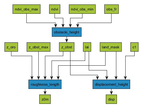
The soil and canopy surface roughness are derived from land cover and NDVI. Land cover classes are used to assign the obstacle height from which surface roughness to momentum (z0,m) is derived. To account for seasonal variation during the growing season, NDVI is used to scale the obstacle height for vegetation.
Under non-neutral conditions also the turbulence generated by buoyancy should be included. The Monin-Obukhov similarity theory (Monin and Obukhov, 1954) is used to describe the effect of buoyancy on the turbulence by means of stability corrections:


Where ψh,obs is the stability correction for heat which is a function of zobs, d and L, the Monin-Obukhov length defined as:

Where:
Ta = air temperature [K]
u<☆>* = friction velocity [m s-1]
H = sensible heat flux (see text below)
The Monin-Obukhov length can be thought of as the height in the boundary layer at which the contribution of shear stress to turbulence is equal to the contribution of buoyancy to turbulence.
Both the aerodynamic resistance under non-neutral conditions and the sensible heat flux, the source of this non-neutral condition, are unknown variables. They can only be solved through an iterative process. A first estimate of the sensible heat flux H using the definitions for ra,soil and ra,canopy under neutral conditions provides a first estimate for the Monin-Obukhov length. The stability corrections ψh,obs are then introduced in an iterative approach. When the iterations are converging, final values of evaporation and transpiration can be calculated. Iterations typically converge after only a small number of iterations (usually approximately 3).
ET conversion to mm
When the aerodynamic resistances are solved, evaporation and transpiration can be calculated. At this stage of the calculations they are still expressed as the available energy for evaporation and transpiration [W m-2], hence the notation: λET, λE, λT in the P-M equation. These are then converted to mm:

Where tday is the number of seconds in a day (86,400) and λ is the latent heat of evaporation which is a function of temperature, λ at 293 K is equal to 2,453,780.
A similar equation can be used for λET, λT. The equation for λ is as follows:

Where c = -2,361 J/kg/C and λ0 = 2,501,000 J/kg
Processing approach
For implementation of the P-M equation in an operational environment using remote sensing data, the P-M equation is dissected to the level of the input data, consisting of 7 (final or intermediate) data components:
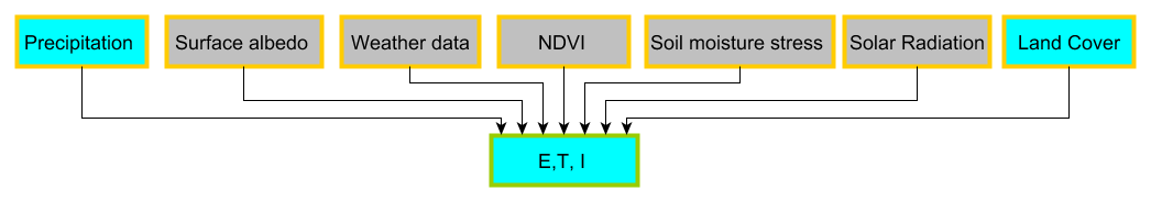
- Solar radiation, Weather data and Precipitation are daily inputs.
- Soil moisture stress, NDVI and Surface albedo are dekadal inputs.
- Calculating E and T requires input from all seven data components while I only requires input from NDVI and Precipitation.
- Land Cover input is used to derive surface roughness and minimum stomatal resistance.
Challenges
Some of the external input data sources (land surface temperature, meteorological data) have a lower spatial resolution than the level 2 and level 3 data components. The spatial variability of these data sources is therefore limited, thereby affecting the resulting E and T data component.
The collection of optical satellite data can be hampered by the presence of clouds, reducing the information on temporal variability. Although both aspects are accommodated for within the data processing chain, its implications should be understood when considering the results: the quality of the E, T, and I data component is a combination of the accuracy of the algorithms and the quality of the external data. The NDVI quality layer is provided to indicate the quality of the external optical satellite data. The LST quality layer is provided to indicate the quality of the external thermal satellite data which is used to compute the soil moisture stress.
Functions and flowcharts
Transpiration functions
| (Intermediate) data component | Functions | Module |
|---|---|---|
| 1 Leaf Area Index | vegetation_cover leaf_area_index |
Leaf |
| 2 Surface Roughness | roughness_length obstacle_height development_height |
Roughness |
| 3 Stress Factors | stress_moisture stress_radiation stress_temperature stress_vpd |
Stress |
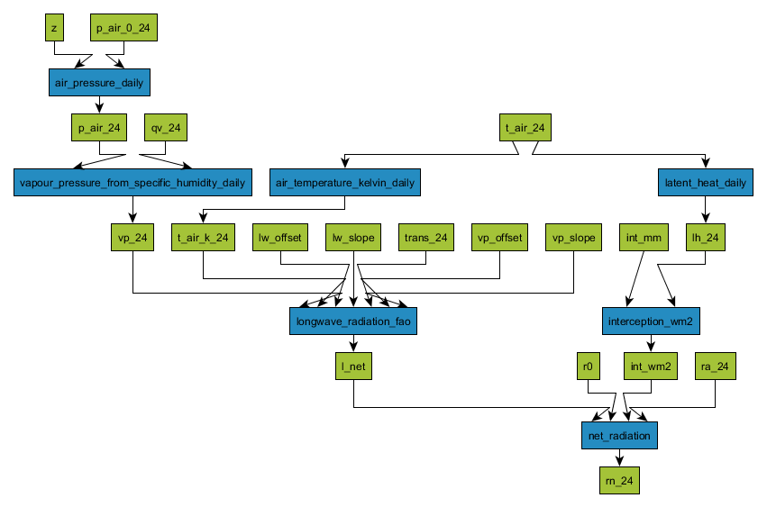
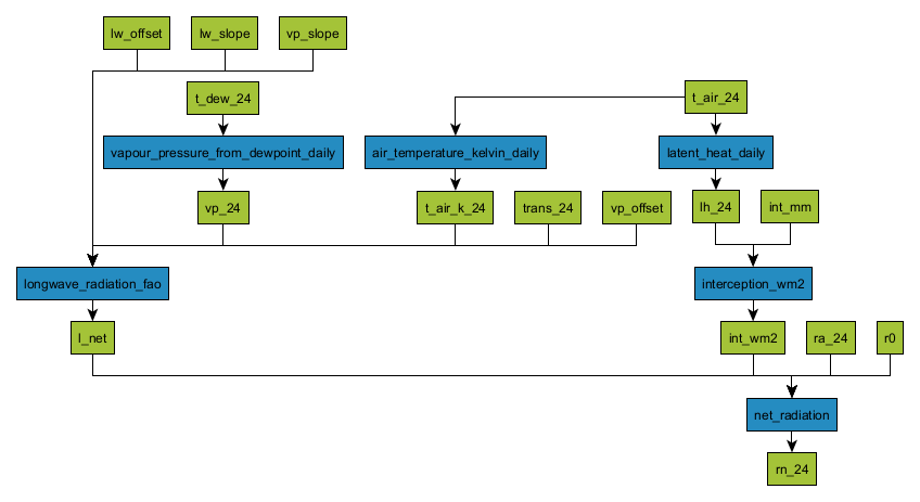
| 4 Net Radiation | latent_heat_daily air_pressure_daily air_temperature_kelvin_daily vapour_pressure_from_specific_humidity_daily vapour_pressure_from_dewpoint_daily |
Meteo |
| 4 Net Radiation | interception_wm2 longwave_radiation_fao net_radiation |
Radiation |
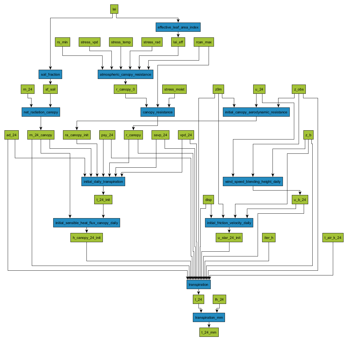
| 5 transpiration | effective_leaf_area_index | Leaf |
| 5 transpiration | soil_fraction net_radiation_canopy |
Radiation |
| 5 transpiration | initial_canopy_aerodynamic_resistance initial_daily_transpiration |
Neutral |
| 5 transpiration | atmospheric_canopy_resistance canopy_resistance |
Resistance |
| 5 transpiration | initial_friction_velocity_daily initial_sensible_heat_flux_canopy_daily transpiration transpiration_mm |
Unstable |
| 5 transpiration | wind_speed_blending_height_daily | Meteo |
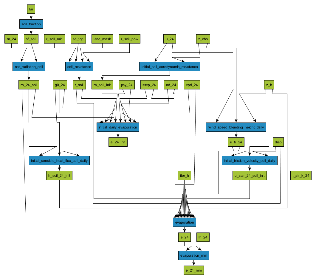
Evaporation functions
| (Intermediate) data component | Functions | Module |
|---|---|---|
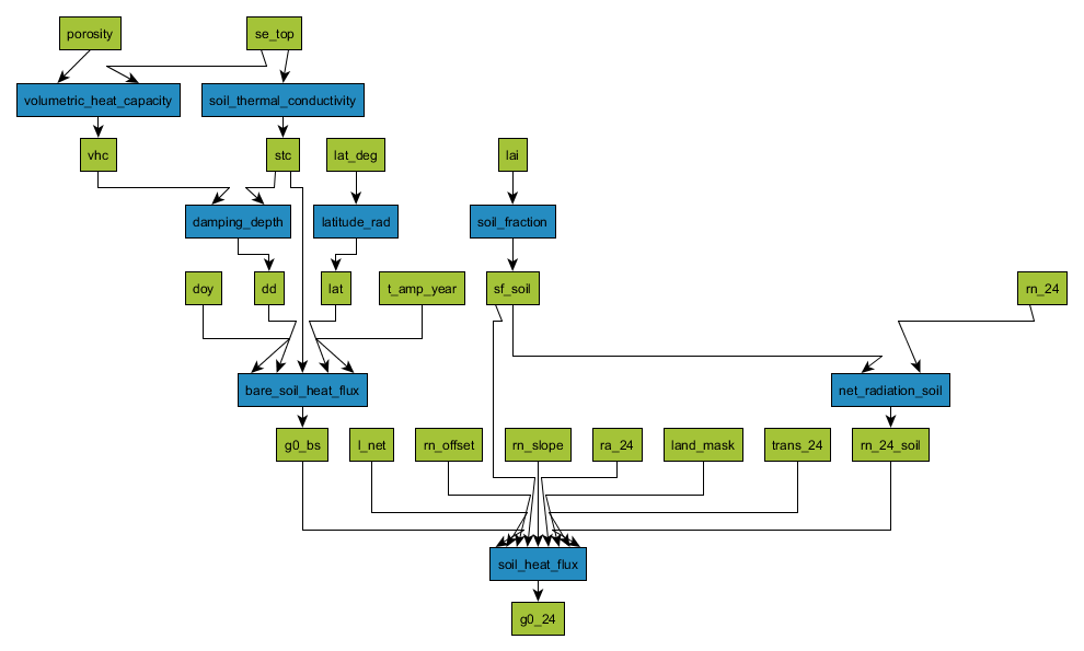
| 6 Soil Heat Flux | bare_soil_heat_flux damping_depth soil_thermal_conductivity volumetric_heat_capacity soil_fraction< br>net_radiation_soil soil_heat_flux |
Radiation |
| 6 Soil Heat Flux | latitude_rad | Solar Radiation |
| 7 evapotranspiration | soil_fraction net_radiation_soil |
Radiation |
| 7 evapotranspiration | soil_resistance | Resistance |
| 7 evapotranspiration | initial_soil_aerodynamic_resistance initial_daily_evaporation |
Neutral |
| 7 evapotranspiration | evaporation evaporation_mm initial_friction_velocity_soil_daily initial_sensible_heat_flux_soil_daily |
Unstable |
| 7 evapotranspiration | wind_speed_blending_height_daily | Meteo |
| 7 evapotranspiration | daily_solar_radiation_toa | Solar_radiation |
Leaf Area Index
Surface Roughness
Stress Factors
Net Radiation NRT (using GEOS-5)
Net Radiation final (using ERA5)
Transpiration
Soil Heat Flux
Evaporation
Updated